For many years, the terminal emulator in Nimble Commander had a pesky bug. The only obvious place where it manifested itself was a particular integration test, and that test managed to be flaky only when running in CI on GitHub. Somehow, I was never able to reproduce the problem locally, despite trying many times and poking the system from different angles.
In the end, I gave up and slapped that test with “[!mayfail]”.
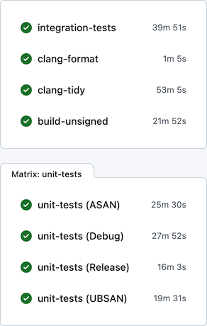
The test in question opened multiple command-line shells and performed very basic operations with them one by one, simply verifying that the terminal buffers eventually reached their expected states. Here’s the source code of that test. This test had me scratching my head for years, filling the CI output with detailed logs that showed no errors. Everything worked “correctly”, but no matter how large the timeouts were, the shells never reached the proper state.
Recently, out of sheer curiosity, I tried feeding this problem to an LLM to see what would happen. It went through many rounds, most of which led to dead ends, for example, proclaiming things like: “The test ‘Test multiple shells in parallel via output’ fails in CI because of slow bash startup caused by ~/.bashrc sourcing on the GitHub Actions macOS runner.”. These “fixes” often sounded plausible, but they didn’t change the actual behaviour – the test still failed. One round, however, the LLM managed to spot an oddity in the logs which I’d been missing all these years because it looked completely innocent.
The logs were filled with boring information that looked like this:
[ShellTask.cpp:290] Starting a new shell: /bin/bash
[ShellTask.cpp:293] Initial work directory: /private/var/folders/p8/qyz0lmpd2mld64f_f4c66y4c0000gn/T/_nc__term__test_/
[ShellTask.cpp:297] Environment:
[ShellTask.cpp:299] 	LANG = en_US.UTF-8
[ShellTask.cpp:299] 	LC_COLLATE = en_US.UTF-8
[ShellTask.cpp:299] 	LC_CTYPE = en_US.UTF-8
[ShellTask.cpp:299] 	LC_MESSAGES = en_US.UTF-8
[ShellTask.cpp:299] 	LC_MONETARY = en_US.UTF-8
[ShellTask.cpp:299] 	LC_NUMERIC = en_US.UTF-8
[ShellTask.cpp:299] 	LC_TIME = en_US.UTF-8
[ShellTask.cpp:299] 	TERM = xterm-256color
[ShellTask.cpp:299] 	TERM_PROGRAM = Nimble_Commander
[ShellTask.cpp:307] posix_openpt(O_RDWR) returned 28 (master_fd)
[ShellTask.cpp:330] ptsname: /dev/ttys009
[ShellTask.cpp:338] slave_fd: 31
[ShellTask.cpp:397] cwd_pipe: 32, 34
[ShellTask.cpp:398] semaphore_pipe: 35, 36
[ShellTask.cpp:408] fork() returned 73394
[ShellTask.cpp:463] prompt_setup:  PROMPT_COMMAND='if [ $$ -eq 73394 ]; then pwd>&20; read sema <&21; fi'
[ShellTask.cpp:607] pwd prompt from shell_pid=73394: /private/var/folders/p8/qyz0lmpd2mld64f_f4c66y4c0000gn/T/_nc__term__test_/
At this point, it’s worth briefly describing how Nimble Commander internally runs command-line shells. When the terminal emulator opens a new shell, it roughly goes through these steps:
-
- prepare the environment (variables, working directory)
- open and configure a pseudo-terminal (posix_openpt(), grantpt(), unlockpt(), ptsname(), open())
- open two pipes that will be used by the prompt command to report the current working directory
- fork() the process
- the master continues setting up state in Nimble Commander itself
- the slave continues configuring the shell process:
- remaps the communication pipes to specific FDs: 20 and 21 (because reasons).
- closes all file handles except [0, 1, 2, 20, 21].
- finally performs execv() to become the shell program requested by the user.
These file descriptors, #20 and #21, allow basic communication between the shell and Nimble Commander. Whenever a user executes “cd /some/directory” in the shell, the associated file panel is expected to pick up the working-directory change and display that path as well. The reporting mechanism is pretty simple under the hood: the shell environment is pre-filled with a variable PROMPT_COMMAND, which contains a command executed each time Bash is about to display a prompt.
The command injected by Nimble Commander looks like this (for Bash; other shells have similar machinery):
if [ $$ -eq 73394 ]; then pwd>&20; read sema <&21; fi
Translated for humans, this means:
If I am the specific process, i.e. the root process of this shell task, then:
    Print the current working directory path to file descriptor #20
    Wait until something can be read from file descriptor #21
FD 20 points to the write end of the pipe that transmits the working directory.
FD 21 points to the read end of the “semaphore” pipe.
Reading from the semaphore pipe provides a basic synchronization mechanism with Nimble Commander – it writes into that pipe to acknowledge that the CWD path has been received.
Now, when a POSIX pipe is opened via pipe(), the file descriptors it creates can have basically any value that happens to be the lowest available number.
So how are they remapped to the fixed numbers 20 and 21?
dup2(int oldfd, int newfd) is at your service, this function does exactly that.
There are a few different cases that dup2() can handle:
-
- if oldfd == newfd, the call is a no-op.
- if newfd is unused, it is opened as a duplicate of oldfd.
- if newfd is a valid descriptor, it’s closed and reopened as a duplicate of oldfd.
Here’s the snippet that performed the remapping:
  if( dup2(I->cwd_pipe[1], g_PromptPipe) != g_PromptPipe ) // #20
    exit(-1);
  if( dup2(I->semaphore_pipe[0], g_SemaphorePipe) != g_SemaphorePipe ) // #21
    exit(-1);
Since all but a few “blessed” FDs are closed before starting the shell program, no explicit closure of the original file descriptors is needed. In case of any error, the child process exits immediately, so if execution continues, it is guaranteed that #20 and #21 are valid file descriptors.
Can you spot the bug?
This code works perfectly well, until the stars align and it no longer does.
Here’s a piece of the logs showing the conditions under which this remapping scheme spectacularly breaks down:
...
[ShellTask.cpp:307] posix_openpt(O_RDWR) returned 13 (master_fd)
[ShellTask.cpp:330] ptsname: /dev/ttys004
[ShellTask.cpp:338] slave_fd: 16
[ShellTask.cpp:397] cwd_pipe: 17, 19
[ShellTask.cpp:398] semaphore_pipe: 20, 21
...
If we substitute the numeric values into the snippet, it becomes this:
  if( dup2(19, 20) != 20 )
    exit(-1);
  if( dup2(20, 21) != 21 )
    exit(-1);
The first dup2() is asked to duplicate #19 as #20.
But #20 is already in use – it’s the read end of the semaphore pipe!
So dup2() silently closes the only existing descriptor for the semaphore pipe’s read end and reopens it as the write end of the CWD pipe.
The second call to dup2() then duplicates that same CWD write descriptor to what was supposed to become the semaphore read descriptor!
So instead of this:
#20 – write CWD
#21 – read Sema
the shell process ends up with this:
#20 – write CWD
#21 – write CWD
And once the shell process executes the prompt command, it tries to read from the write end of the pipe and deadlocks forever.
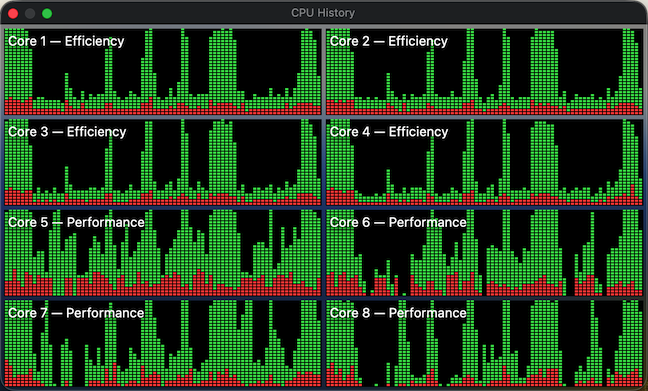
Normally, the file descriptors would have much higher values, so they wouldn’t clobber each other. In this particular test, however, the process had a very pristine state and allocated file descriptors starting from very low numbers. Gradually opening multiple shells one by one, it eventually stepped on its own toes:
[ShellTask.cpp:307] posix_openpt(O_RDWR) returned 4 (master_fd)
[ShellTask.cpp:330] ptsname: /dev/ttys000
[ShellTask.cpp:338] slave_fd: 5
[ShellTask.cpp:397] cwd_pipe: 6, 7
[ShellTask.cpp:398] semaphore_pipe: 8, 9
[ShellTask.cpp:307] posix_openpt(O_RDWR) returned 5 (master_fd)
[ShellTask.cpp:330] ptsname: /dev/ttys001
[ShellTask.cpp:338] slave_fd: 7
[ShellTask.cpp:397] cwd_pipe: 8, 10
[ShellTask.cpp:398] semaphore_pipe: 11, 12
[ShellTask.cpp:307] posix_openpt(O_RDWR) returned 7 (master_fd)
[ShellTask.cpp:330] ptsname: /dev/ttys002
[ShellTask.cpp:338] slave_fd: 10
[ShellTask.cpp:397] cwd_pipe: 11, 13
[ShellTask.cpp:398] semaphore_pipe: 14, 15
[ShellTask.cpp:307] posix_openpt(O_RDWR) returned 10 (master_fd)
[ShellTask.cpp:330] ptsname: /dev/ttys003
[ShellTask.cpp:338] slave_fd: 13
[ShellTask.cpp:397] cwd_pipe: 14, 16
[ShellTask.cpp:398] semaphore_pipe: 17, 18
[ShellTask.cpp:307] posix_openpt(O_RDWR) returned 13 (master_fd)
[ShellTask.cpp:330] ptsname: /dev/ttys004
[ShellTask.cpp:338] slave_fd: 16
[ShellTask.cpp:397] cwd_pipe: 17, 19
[ShellTask.cpp:398] semaphore_pipe: 20, 21. <<<<<< BOOM!
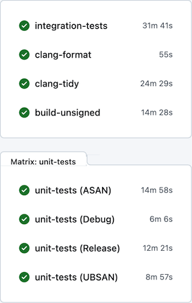
The fix was fairly straightforward: just check for potential overlaps between the source and target file descriptor numbers before remapping.
If there’s any moral to this bug of mine, it’s probably this:
-
- No matter how seasoned you are, you will sometimes make silly mistakes.
- APIs with implicit side effects are utterly evil.
- There’s no harm in trying every tool at your disposal, even if they often hallucinate.