Drawing a Hosek-Wilkie sky on CPU, fast

While working on my toy software rasterizer, at some point I decided to try rendering a skybox using cube maps. Loading and drawing a pre-existing environment cube map as 12 triangles proved to be easy and boring. Next, I looked into generating the skybox programmatically on the fly during each frame. The first attempt used the Preetham daylight model. It worked, but I couldn’t tune it well enough to produce good-looking results for a dynamic sky with the Sun moving in real time from dawn till dusk. This paper explores the issues well: “A Critical Review of the Preetham Skylight Model”. Next attempt used the Hosek-Wilkie sky model (paper, presentation), which produced much more convincing results.

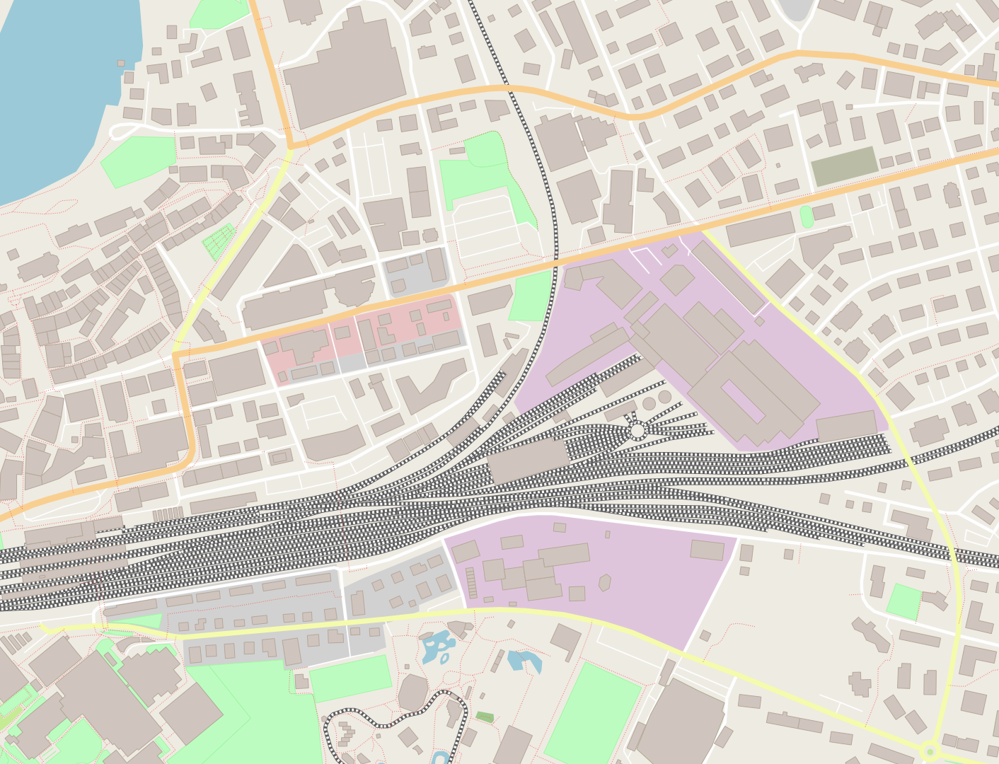
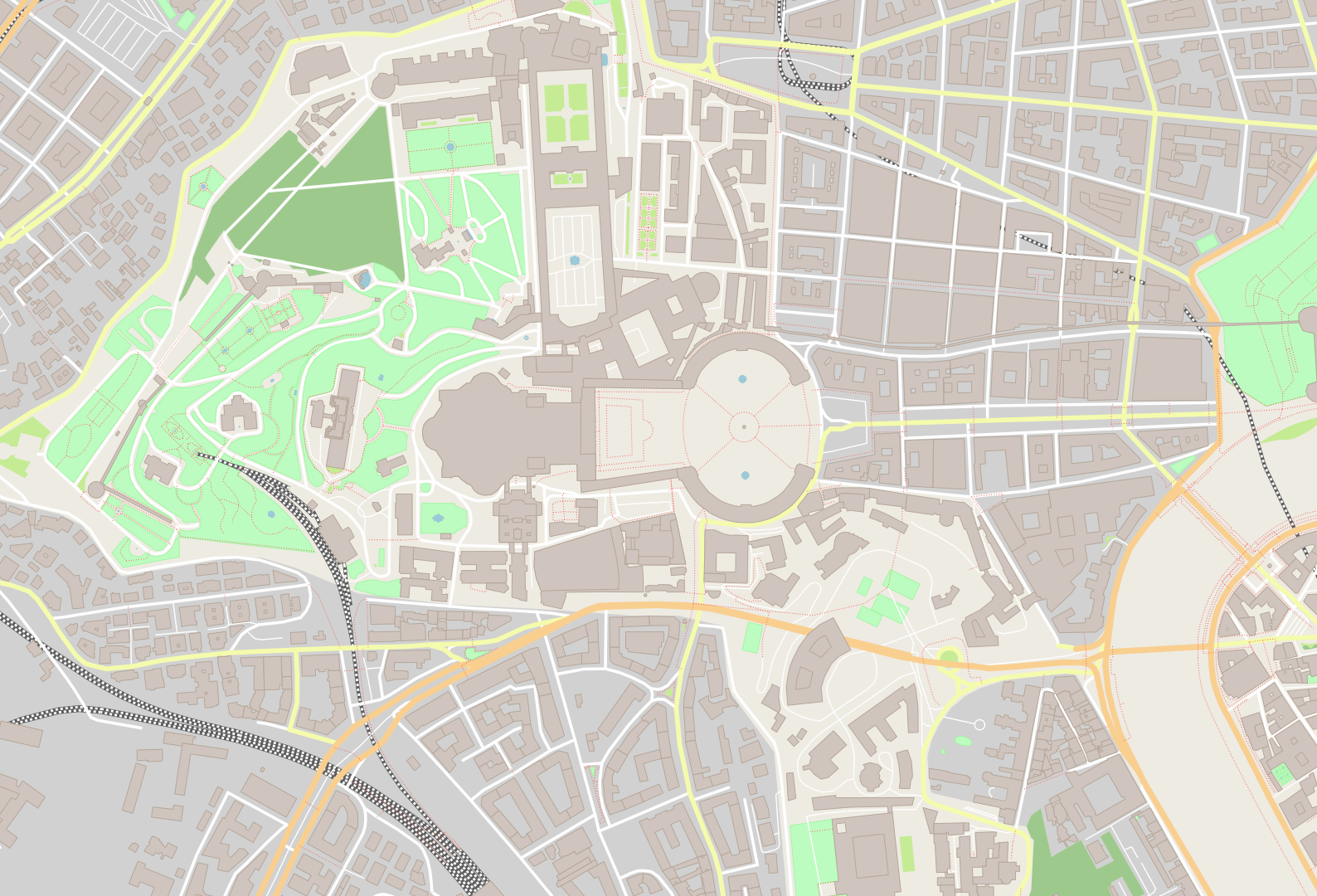
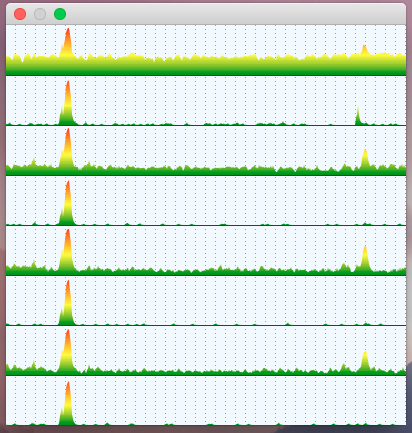
This model allows sampling sky radiance to build an image like this:

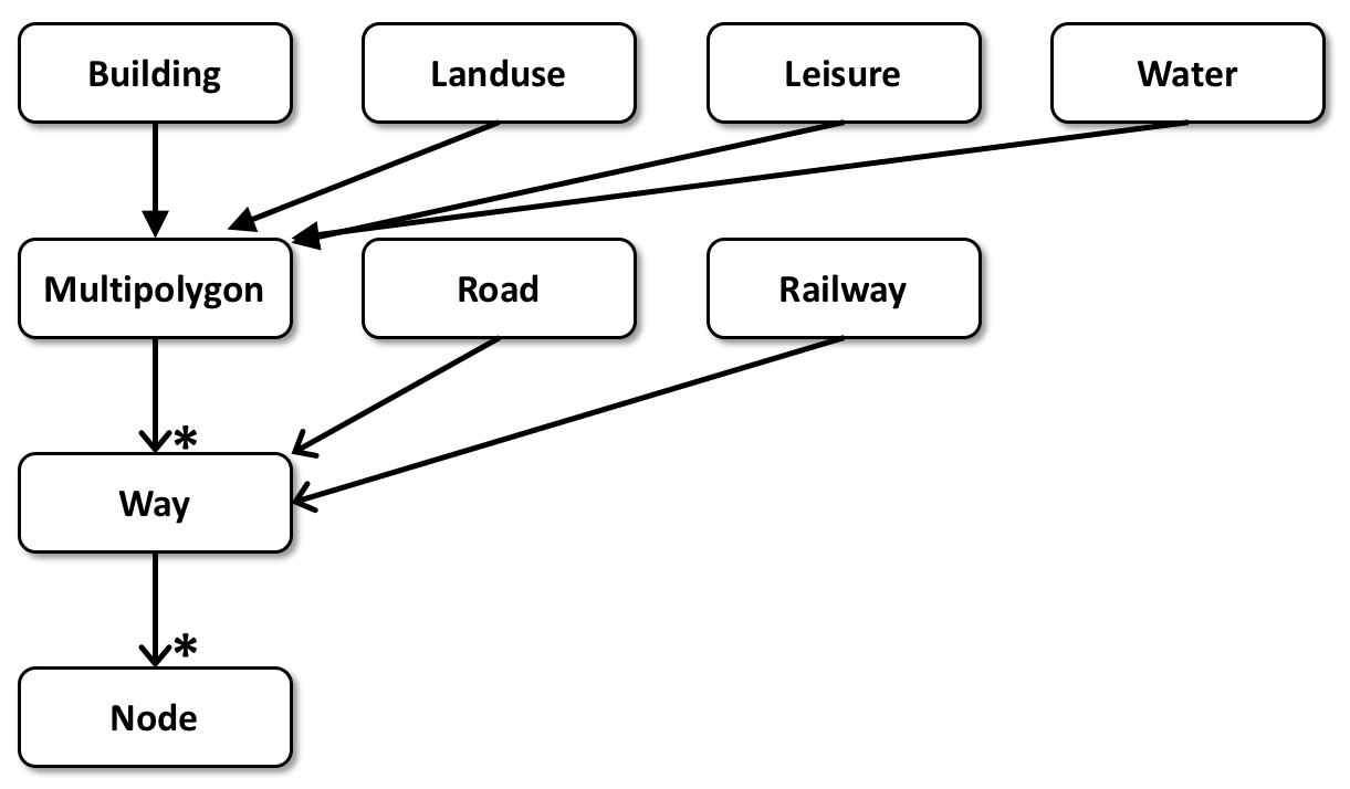
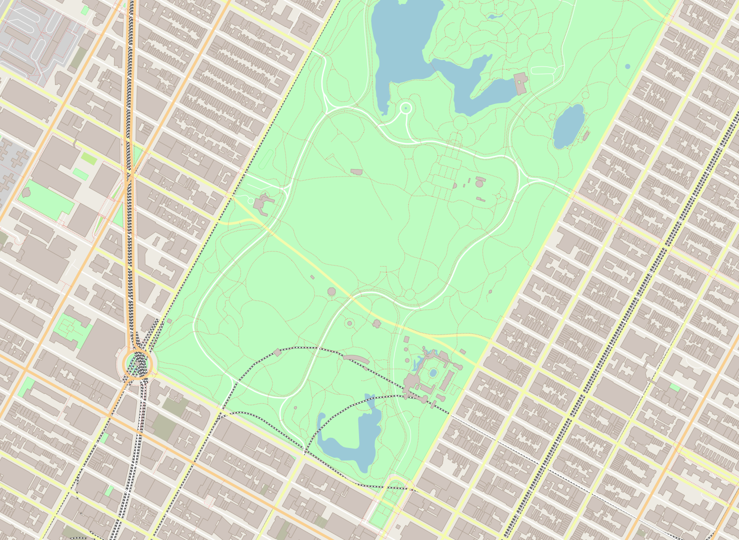
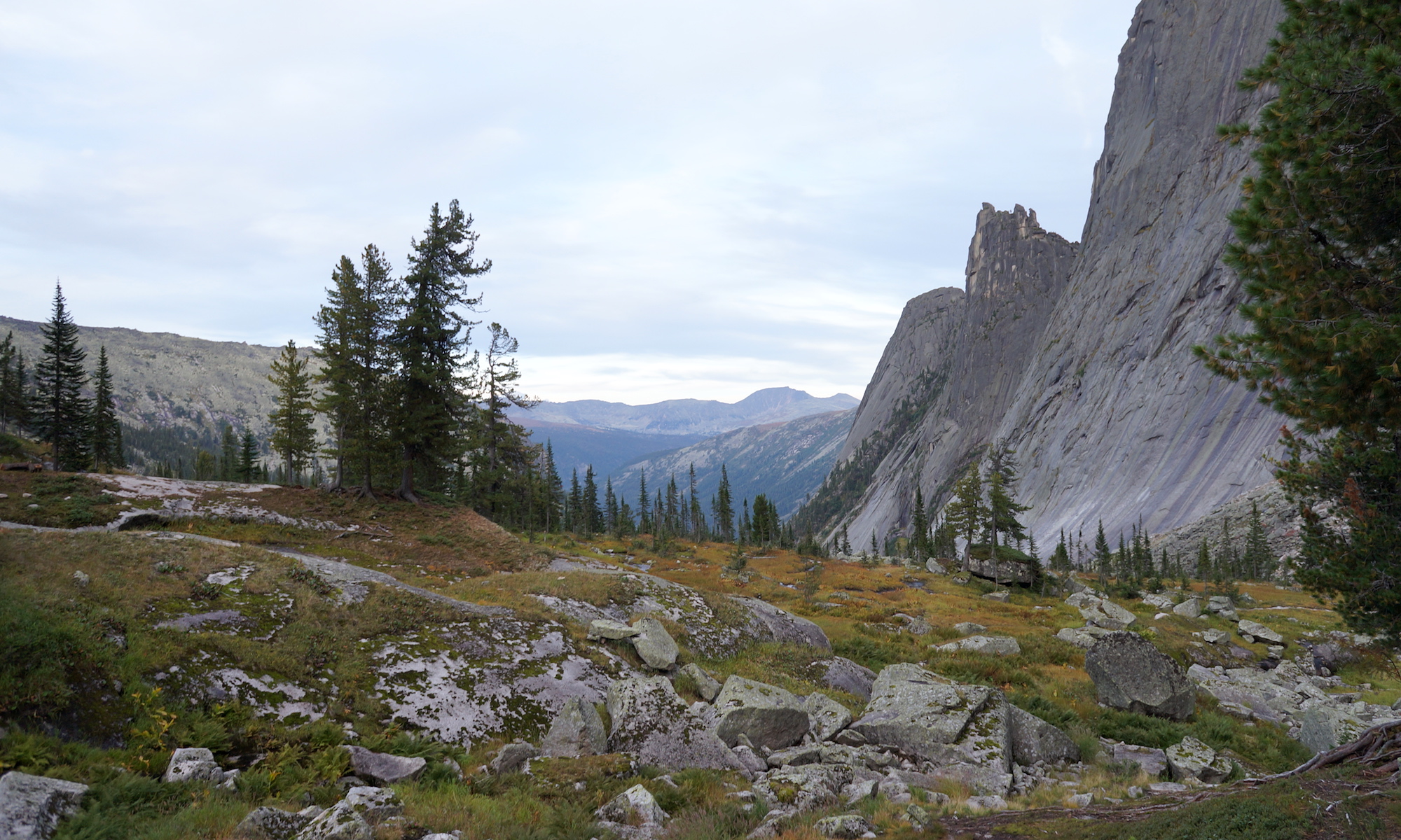
When combined with a visualization of a moving Sun and rendered for five cube-map faces each frame, it results in a lively sky background like this:

This video shows the Skybox example from the NIH2 software renderer, which runs at ~150 FPS at 720p on an Apple M1 CPU.

This blogpost summarizes the experience of running the Hosek-Wilkie sky model on the CPU and iteratively optimizing the implementation enough for semi real-time use cases. It also provides a distilled version of the source code detached from the software renderer. The code is written in Rust, but this doesn’t matter much, as the logic behind the optimizations is equally applicable to any compiled language.

For simplicity, the implementation builds only a single cube-map face (negative Z). Since the sky model is defined only for Sun directions with Y>=0, only the top half of this face is filled. Extending the logic for other faces is pretty straightforward, but makes the code hairier, so they were omitted.

The optimizations focus on single-threaded performance, as building multiple faces can be trivially parallelized across threads. A resolution of 1024×512 was chosen for benchmarking each iteration of the code, measurements were done on the base Apple M1 CPU.

V0 – Initial implementation

The sky model has two kinds of inputs:

    • Per entire sky dome (during model initialization):
      • Turbidity [1..10] – measure of aerosol content in the air
      • Ground albedo [0..1 x 3] – fraction of sunlight reflected by the ground
      • Solar elevation [0°..90°] – how high the Sun is
    • Per view direction (during sampling):
      • Theta θ [0°..90°] – view angle from the zenith
      • Gamma γ [0°..180°] – angle between the view direction and the Sun

Conceptually, building a single cube-map face consists of the following steps:

    • Initialize the sky model (can be shared across faces)
    • For each pixel on the face:
      • Compute θ and γ
      • Sample the model with (θ, γ) three times (once per RGB channel)
      • Tone-map, convert to sRGB, and write out as U8 x 3

Sky model initialization is performed once per frame and is very cheap. It mainly consists of evaluating equation (11) a few times on the table data and lerping between the results.

θ and γ are computed from pixel coordinates (x, y) as follows:

let u: f32 = 2.0 * (x as f32 + 0.5) / (width as f32) - 1.0; // [-1, 1]         
let v: f32 = ((height - 1 - y) as f32 + 0.5) / (height as f32); // [0, 1]
let dir: Vec3 = Vec3::new(u, v, -1.0).normalize(); // ZNeg => Z=-1
let theta: f32 = dir.y.acos(); // view angle from zenith
let cos_gamma: f32 = dir.dot(sun_direction);
let gamma: f32 = cos_gamma.acos(); // angle between view direction and sun


Sampling the model is done by implementing the equations (8, 9) directly:

pub fn f(&self, theta: f32, gamma: f32) -> (f32, f32, f32) {
  let chi = |g: f32, a: f32| -> f32 {
    let num: f32 = 1.0 + a.cos().powi(2);
    let denom: f32 = (1.0 + g.powi(2) - 2.0 * g * a.cos()).powf(3.0 / 2.0);
    num / denom
  };
  let eval = |p: [f32; 9], theta: f32, gamma: f32| -> f32 {
    let a: f32 = p[0];
    // ...
    let i: f32 = p[8];
    let term1: f32 = 1.0 + a * (b / (theta.cos() + 0.01)).exp();
    let term2: f32 = c + d * (e * gamma).exp() + f * gamma.cos().powi(2) +
      g * chi(i, gamma) + h * theta.cos().sqrt();
    term1 * term2
    };
  let f0: f32 = eval(self.distribution[0], theta, gamma);
  let f1: f32 = eval(self.distribution[1], theta, gamma);
  let f2: f32 = eval(self.distribution[2], theta, gamma);
  (f0 * self.radiance[0], f1 * self.radiance[1], f2 * self.radiance[2])
}


For tone mapping I used Reinhard since it’s simple and robust. Gamma correction and clamping are applied before writing out a pixel:

  // ...
  let f: (f32, f32, f32) = sky.f(theta, gamma); // sample the radiance
  let c: (f32, f32, f32) = linear_to_rgb(f); // convert to display sRGB space
  // Write out as u8 RGB
  let idx: usize = y * width + x; // pixel index
  pixels[idx * 3 + 0] = (c.0 * 255.0).clamp(0.0, 255.0) as u8;
  pixels[idx * 3 + 1] = (c.1 * 255.0).clamp(0.0, 255.0) as u8;
  pixels[idx * 3 + 2] = (c.2 * 255.0).clamp(0.0, 255.0) as u8;
  // ...
        
fn to_srgb(c: (f32, f32, f32)) -> (f32, f32, f32) {
  let encode = |x: f32| {
    if x <= 0.0031308 {
      12.92 * x
    } else {
      1.055 * x.powf(1.0 / 2.4) - 0.055
    }
  };
  (encode(c.0), encode(c.1), encode(c.2))
}

fn tonemap_reinhard(rgb: (f32, f32, f32), exposure: f32, white: f32) ->
  (f32, f32, f32) {
  let r: f32 = rgb.0 * exposure;
  let g: f32 = rgb.1 * exposure;
  let b: f32 = rgb.2 * exposure;
  let y: f32 = 0.2126 * r + 0.7152 * g + 0.0722 * b;
  let s: f32 = (1.0 + y / (white * white)) / (1.0 + y);
  (r * s, g * s, b * s)
}

fn linear_to_rgb(c: (f32, f32, f32)) -> (f32, f32, f32) {
  let exposure: f32 = 0.5;
  let white_point: f32 = 14.0;
  let exposed: (f32, f32, f32) = tonemap_reinhard(c, exposure, white_point);
  let display: (f32, f32, f32) = to_srgb(exposed);
  display
}


Result: this version works, but it takes ~46ms to build a single face. Too slow…

V1 – Less wasteful computation

The amount of work the poor old scalar CPU has to perform per pixel is no joke. Worse still, compilers (including rustc) are constrained by strict IEEE floating-point semantics, which prevents many otherwise valid optimizations. However, it is possible to manually simplify parts of the formulas and hoist redundant computations:

    • cos(θ) and cos(γ) are already available, there’s no need to re-calculate them again inside the function body
    • v.powf(3.0 / 2.0) is mathematically equivalent to v * v.sqrt(), which is much cheaper
    • v.powi(2) is equivalent to v * v, in case the compiler fails to expand it

Result: these simple transformations reduce the compute time down to ~28ms.

V2 – Per-pixel SIMD

Staring at this snippet for long enough:

    let f0: f32 = eval(self.distribution[0]);
    let f1: f32 = eval(self.distribution[1]);
    let f2: f32 = eval(self.distribution[2]);

… eventually raises the question – since we’re doing the same computation three times, just with different input data, why not do all three in parallel?

Of course, there are no SIMD registers with three lanes, but nothing prevents from using a fourth throwaway lane for free. Effectively, running the formulas (8, 9) for RGBX, where the distribution and radiance values for the fourth lane are zeroed out.

A direct translation of the sampling function to 4-way SIMD looks like this:

pub fn f(&self, theta: f32, gamma: f32, theta_cos: f32, gamma_cos: f32) -> (f32, f32, f32) {
  let a: F32x4 = F32x4::load(self.distribution4[0]);
  ...
  let i: F32x4 = F32x4::load(self.distribution4[8]);
  let one: F32x4 = F32x4::splat(1.0);
  let two: F32x4 = F32x4::splat(2.0);
  let zero_zero_one: F32x4 = F32x4::splat(0.01);
  let gamma: F32x4 = F32x4::splat(gamma);
  let theta_cos: F32x4 = F32x4::splat(theta_cos);
  let gamma_cos: F32x4 = F32x4::splat(gamma_cos);
  let radiance: F32x4 = F32x4::load(self.radiance4);
  let term1: F32x4 = (b / (theta_cos + zero_zero_one)).exp() * a + one;
  let chi_num: F32x4 = one + gamma_cos * gamma_cos;
  let chi_denom: F32x4 = one + i * (i - gamma_cos * two);
  let chi: F32x4 = chi_num / (chi_denom * chi_denom.sqrt());
  let term2: F32x4 = c + d * (e * gamma).exp() + f * gamma_cos * gamma_cos +
    g * chi + h * theta_cos.sqrt();
  let c: F32x4 = (term1 * term2) * radiance;
  let c4: [f32; 4] = c.store();
  (c4[0], c4[1], c4[2])
}

Here I use a custom F32x4 SIMD type that provides trig and pow/exp/log operations, but really any decent SIMD library would do. I’m mostly using ARM64, but also want the code to run on AMD64, so a 4-wide type is the common denominator.

Result: this version takes the previous ~28ms down to ~26ms. Meh, rather underwhelming. It clearly demonstrates a well-known truth – effective SIMD requires rethinking both data layout and function interfaces. Otherwise, the ceremony of setting up SIMD computation and getting the results back nullifies any gains from the parallel compute.

V3 – Per-row SIMD

The next step was to go into full SIMD. Drop the per-pixel approach entirely and instead perform the computation per rows, separately for the R, G, and B channels. With width=1024, this means first writing out (cos(θ), γ, cos(γ)) for the entire row (1024 x 3 x 4b = 12Kb), and then calculating the formulas (8, 9) from the paper and writing them into three output arrays (1024 x 3 x 4b = 12Kb). Since the size of the scratchpad arrays is about 24Kb, the CPU should rarely touch memory outside the L1 cache:

// Per-row scratch space
let mut theta_cos_row: Vec<f32> = vec![0.0; width];
let mut gamma_cos_row: Vec<f32> = vec![0.0; width];
let mut gamma_row: Vec<f32> = vec![0.0; width];
let mut r_row: Vec<f32> = vec![0.0; width];
let mut g_row: Vec<f32> = vec![0.0; width];
let mut b_row: Vec<f32> = vec![0.0; width];

//...

// Calculate radiance per each channel, entire row at a time
sky.f_simd_r(&gamma_row, &theta_cos_row, &gamma_cos_row, &mut r_row);
sky.f_simd_g(&gamma_row, &theta_cos_row, &gamma_cos_row, &mut g_row);
sky.f_simd_b(&gamma_row, &theta_cos_row, &gamma_cos_row, &mut b_row);

The function interface changes accordingly – it now accepts spans of input arrays and a span of an output array. The internal logic remains the same, but it operates on chunks of 4 input values, passing them through the transformation and writing out 4 results per iteration:

fn f_simd_channel<const CHANNEL: usize>(
  &self,
  gamma: &[f32],
  theta_cos: &[f32],
  gamma_cos: &[f32],
  output: &mut [f32]) {
  let gamma: *const f32 = gamma.as_ptr();
  let theta_cos: *const f32 = theta_cos.as_ptr();
  let gamma_cos: *const f32 = gamma_cos.as_ptr();
  let output: *mut f32 = output.as_mut_ptr();
  let a: F32x4 = F32x4::splat(self.distribution[CHANNEL][0]);
  // ...
  let i: F32x4 = F32x4::splat(self.distribution[CHANNEL][8]);
  let one: F32x4 = F32x4::splat(1.0);
  let two: F32x4 = F32x4::splat(2.0);
  let zero_zero_one: F32x4 = F32x4::splat(0.01);
  let radiance: F32x4 = F32x4::splat(self.radiance[CHANNEL]);
  for idx in (0..=len - 4).step_by(4) {
    let gamma: F32x4 = F32x4::load(unsafe {*(gamma.add(idx) as *const [f32; 4])});
    let theta_cos: F32x4 = F32x4::load(unsafe {*(theta_cos.add(idx) as *const [f32; 4])});
    let gamma_cos: F32x4 = F32x4::load(unsafe {*(gamma_cos.add(idx) as *const [f32; 4])});
    let term1: F32x4 = (b / (theta_cos + zero_zero_one)).exp() * a + one;
    let chi_num: F32x4 = one + gamma_cos * gamma_cos;
    let chi_denom: F32x4 = one + i * (i - gamma_cos * two);
    let chi: F32x4 = chi_num / (chi_denom * chi_denom.sqrt());
    let term2: F32x4 = c + d * (e * gamma).exp() + f * gamma_cos * gamma_cos + g * chi + h * theta_cos.sqrt();
    let c: F32x4 = (term1 * term2) * radiance;
    c.store_to(unsafe { &mut *(output.add(idx) as *mut [f32; 4]) });
  }
}

Result: this data-layout transformation cuts the runtime from ~26ms to ~13ms. In other words, it is twice as fast while conceptually doing more work in the process, since inputs and outputs are first written to scratch arrays instead of being consumed immediately one by one.

V4 – FMA and raw pointer arithmetic

Now that the implementation operates in SIMD intrinsics, it becomes possible to save a few more instructions by using fused multiply-add (FMA) where applicable. The assembly listing also showed some unnecessary checks around loop iteration and pointer arithmetic; this can be fixed by re-writing the code to be as primitive as possible:

fn f_simd_channel<const CHANNEL: usize>(
  &self,
  gamma: &[f32],
  theta_cos: &[f32],
  gamma_cos: &[f32],
  output: &mut [f32]) {
  let mut gamma_ptr: *const f32 = gamma.as_ptr();
  let mut theta_cos_ptr: *const f32 = theta_cos.as_ptr();
  let mut gamma_cos_ptr: *const f32 = gamma_cos.as_ptr();
  let mut output_ptr: *mut f32 = output.as_mut_ptr();
  let a: F32x4 = F32x4::splat(self.distribution[CHANNEL][0]);
  // ...
  let i: F32x4 = F32x4::splat(self.distribution[CHANNEL][8]);
  let one: F32x4 = F32x4::splat(1.0);
  let minus_two: F32x4 = F32x4::splat(-2.0);
  let zero_zero_one: F32x4 = F32x4::splat(0.01);
  let radiance: F32x4 = F32x4::splat(self.radiance[CHANNEL]);
  let steps: usize = len / 4;
  for _idx in 0..steps {
    let gamma: F32x4 = F32x4::load(unsafe { *(gamma_ptr as *const [f32; 4]) });
    let theta_cos: F32x4 = F32x4::load(unsafe { *(theta_cos_ptr as *const [f32; 4]) });
    let gamma_cos: F32x4 = F32x4::load(unsafe { *(gamma_cos_ptr as *const [f32; 4]) });
    let term1: F32x4 = (b / (theta_cos + zero_zero_one)).exp().fma(a, one);
    let chi_num: F32x4 = gamma_cos.fma(gamma_cos, one);
    let chi_denom: F32x4 = gamma_cos.fma(minus_two, i).fma(i, one);
    let chi: F32x4 = chi_num / (chi_denom * chi_denom.sqrt());
    let term2: F32x4 = theta_cos
        .sqrt()
        .fma(h, (f * gamma_cos).fma(gamma_cos, g.fma(chi, (e * gamma).exp().fma(d, c))));
    let channel_radiance: F32x4 = (term1 * term2) * radiance;
    channel_radiance.store_to(unsafe { &mut *(output_ptr as *mut [f32; 4]) });
    gamma_ptr = unsafe { gamma_ptr.add(4) };
    theta_cos_ptr = unsafe { theta_cos_ptr.add(4) };
    gamma_cos_ptr = unsafe { gamma_cos_ptr.add(4) };
    output_ptr = unsafe { output_ptr.add(4) };
  }
}

With these changes, the core of the implementation turns into a large loop with one conditional jump. The assembly output becomes a wall of branchless 4-wide vector operations, beautiful!

Result: these tweaks shave off another ~1ms from the runtime, bringing it down to ~12ms.

V5 – Computing theta and gamma with SIMD

At this point there are no more low-hanging fruits in the Hosek-Wilkie sky sampling itself; the scaffolding around it became the bottleneck instead. The calculation of theta and gamma, while not super expensive, can still be accelerated by deriving 4 triplets at a time. Instead of recalculating (u, v) from (x, y) per-pixel, the initial direction vector and the dX/dY stepping constants are computed once. Next, updating the direction component, while stepping through 4 values, is then done via a single add instruction:

for x in (0..width).step_by(4) {
  // normalize the components of the direction vector
  let recip_len_sqrt: F32x4 = vec_x_4.fma(vec_x_4, vec_y2_z2_4).rsqrt();
  let normalized_vec_x_4: F32x4 = vec_x_4 * recip_len_sqrt;
  let normalized_vec_y_4: F32x4 = vec_y_4 * recip_len_sqrt;
  let normalized_vec_z_4: F32x4 = vec_z_4 * recip_len_sqrt;
  // cos(theta) - cos(angle between the zenith and the view direction)
  let theta_cos_4: F32x4 = normalized_vec_y_4;
  // gamma_cos = dot(dir, sun_dir).clamp(-1.0, 1.0);
  let gamma_cos_4: F32x4 = (normalized_vec_x_4 * sun_dir_x_4
    + normalized_vec_y_4 * sun_dir_y_4
    + normalized_vec_z_4 * sun_dir_z_4)
      .min(F32x4::splat(1.0))
      .max(F32x4::splat(-1.0));
  // gamma - angle between the view direction and the Sun
  let gamma_4: F32x4 = gamma_cos_4.acos();
  theta_cos_4.store_to(unsafe {&mut *(theta_cos_row.as_mut_ptr().add(x) as *mut [f32; 4])});
  gamma_cos_4.store_to(unsafe {&mut *(gamma_cos_row.as_mut_ptr().add(x) as *mut [f32; 4])});
  gamma_4.store_to(unsafe {&mut *(gamma_row.as_mut_ptr().add(x) as *mut [f32; 4])});
  vec_x_4 += dir_dx_x_4; // step the direction vector forward by 4 texels
}

Result: calculating four (cos(θ), γ, cos(γ)) triplets at a time removes another ~1ms, now at ~11ms. Likely this part can be optimized a bit further, but it already feels like a territory of diminishing returns.

V6 – Tone mapping and gamma correction in SIMD

The only scalar part left is processing the HDR output from the Hosek-Wilkie sky model. This stage also needs to be re-written to take 3 per-component arrays and produce a single SDR RGB array. The operation is somewhat awkward – the input data are laid out per component (RRRR… GGGG… BBBB…), while the output must be interleaved per pixel (rgbrgbrgbrgb…). Still, with the help of a few useful ARM64 instructions and LLVM’s excellent backend optimizer, the result is surprisingly good.

Another important ingredient in making this fast is CHEATING:

    • For skybox rendering, the sRGB transfer function can be simplified to a power function powf(1.0/2.2) without visually noticeable difference
    • powf(1.0/2.2) is close enough to powf(1.0/2.0), which is just sqrt(), i.e. a single CPU instruction, voila!

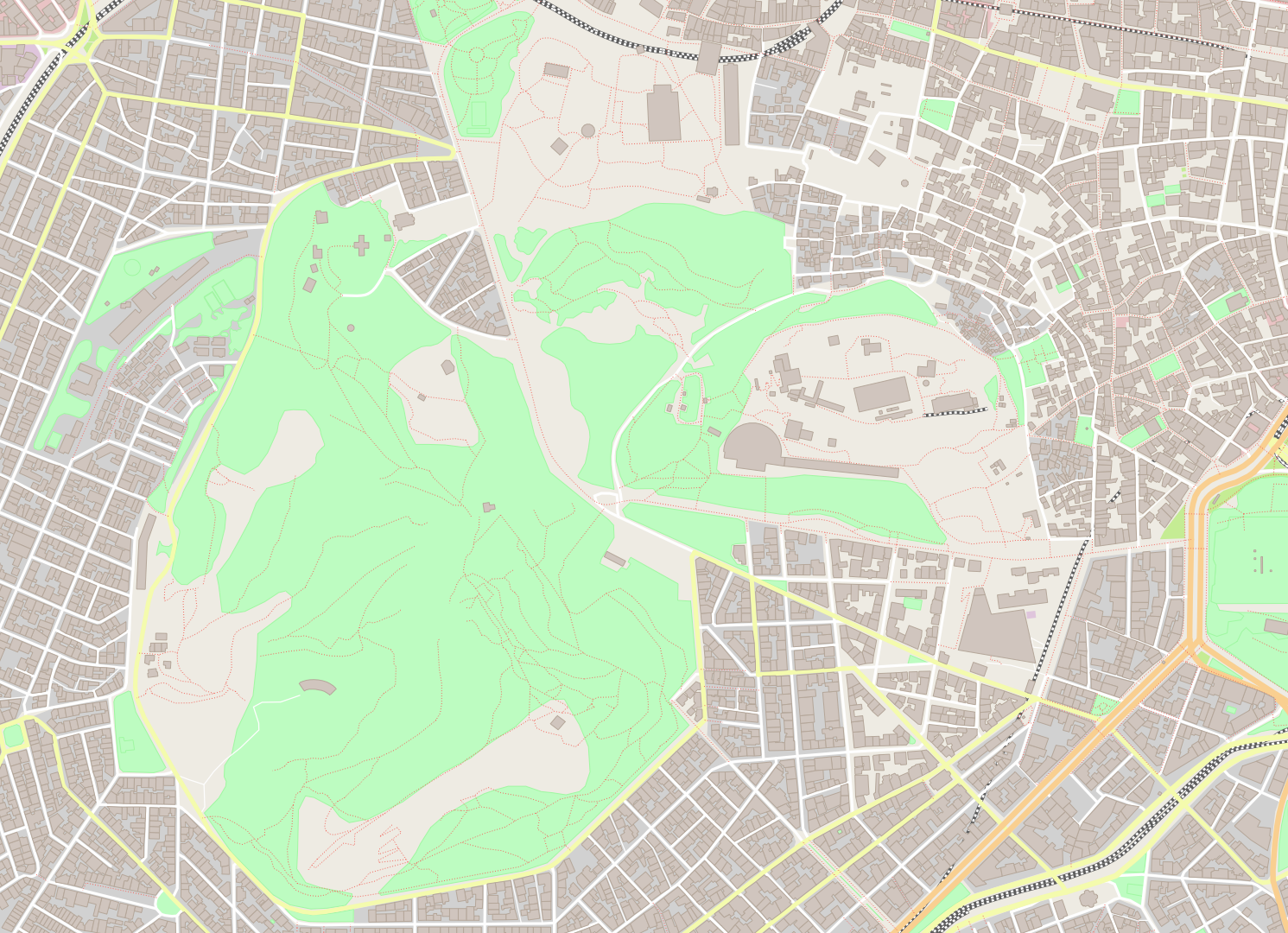
It is also convenient to inject a bit of noise into this post-processing stage to reduce visible banding (before and after debanding):

The combined and SIMDified version of post-processing looks like this:

pub fn map(&self, r: &[f32], g: &[f32], b: &[f32],
  texels24: &mut [u8], y: usize) {
  let mut r_ptr: *const f32 = r.as_ptr();
  let mut g_ptr: *const f32 = g.as_ptr();
  let mut b_ptr: *const f32 = b.as_ptr();
  let mut output_ptr: *mut u8 = texels24.as_mut_ptr();
  let steps: usize = r.len() / 4;
  let zero: F32x4 = F32x4::splat(0.0);
  let one: F32x4 = F32x4::splat(1.0);
  let to_255: F32x4 = F32x4::splat(255.0);
  let exposure: F32x4 = self.exposure;
  let luma_weights_r: F32x4 = self.luma_weights_r;
  let luma_weights_g: F32x4 = self.luma_weights_g;
  let luma_weights_b: F32x4 = self.luma_weights_b;
  let inv_white_point2: F32x4 = self.inv_white_point2;
  let noise_r: F32x4 = F32x4::load(NOISE_TABLE[(y + 0) % 16]);
  let noise_g: F32x4 = F32x4::load(NOISE_TABLE[(y + 1) % 16]);
  let noise_b: F32x4 = F32x4::load(NOISE_TABLE[(y + 2) % 16]);
  for _idx in 0..steps {
    // Load inputs in sRGB primaries with a linear gamma ramp
    let r: F32x4 = F32x4::load(unsafe { *(r_ptr as *const [f32; 4]) });
    let g: F32x4 = F32x4::load(unsafe { *(g_ptr as *const [f32; 4]) });
    let b: F32x4 = F32x4::load(unsafe { *(b_ptr as *const [f32; 4]) });
    // Expose
    let re: F32x4 = r * exposure;
    let ge: F32x4 = g * exposure;
    let be: F32x4 = b * exposure;
    // Calculate luminance: dot(rgb, luma_weights)
    let luma: F32x4 = re * luma_weights_r + ge * luma_weights_g + be * luma_weights_b;
    // Calculate white scale: (1 + luma / white_point^2) / (1 + luma)
    let scale: F32x4 = luma.fma(inv_white_point2, one) / (one + luma);
    // Map to SDR
    let rt: F32x4 = re * scale;
    let gt: F32x4 = ge * scale;
    let bt: F32x4 = be * scale;
    // Gamma-correction: v = v^(1.0/2.0)
    let rc: F32x4 = rt.sqrt();
    let gc: F32x4 = gt.sqrt();
    let bc: F32x4 = bt.sqrt();
    // Apply some noise for dithering
    let r_final: F32x4 = rc + noise_r;
    let g_final: F32x4 = gc + noise_g;
    let b_final: F32x4 = bc + noise_b;
    // Clamp the values to [0.0, 1.0] and convert to [0.0, 255.0]
    let r_out: F32x4 = r_final.min(one).max(zero) * to_255;
    let g_out: F32x4 = g_final.min(one).max(zero) * to_255;
    let b_out: F32x4 = b_final.min(one).max(zero) * to_255;
    // Convert to integers [0, 255]
    let r_u32: [u32; 4] = r_out.to_u32().store();
    let g_u32: [u32; 4] = g_out.to_u32().store();
    let b_u32: [u32; 4] = b_out.to_u32().store();
    // Store the output texels
    unsafe {
      *output_ptr.add(0) = r_u32[0] as u8;
      *output_ptr.add(1) = g_u32[0] as u8;
      *output_ptr.add(2) = b_u32[0] as u8;
      *output_ptr.add(3) = r_u32[1] as u8;
      *output_ptr.add(4) = g_u32[1] as u8;
      *output_ptr.add(5) = b_u32[1] as u8;
      *output_ptr.add(6) = r_u32[2] as u8;
      *output_ptr.add(7) = g_u32[2] as u8;
      *output_ptr.add(8) = b_u32[2] as u8;
      *output_ptr.add(9) = r_u32[3] as u8;
      *output_ptr.add(10) = g_u32[3] as u8;
      *output_ptr.add(11) = b_u32[3] as u8;
    };
    // Advance the input/output pointers
    r_ptr = unsafe { r_ptr.add(4) };
    g_ptr = unsafe { g_ptr.add(4) };
    b_ptr = unsafe { b_ptr.add(4) };
    output_ptr = unsafe { output_ptr.add(12) };
  }
}

Again, the main loop becomes a branchless wall of 4-wide vector operations.

Result: this change pushes the time down to ~4ms. At this point, the Hosek-Wilkie skybox can be regenerated comfortably every frame, allowing smooth real-time Sun movement.

Summary

Overall optimization progress from version to version is summarized in the table below:

Initial version ~46ms
Less wasteful computation ~28ms
Per-pixel SIMD ~26ms
Per-row SIMD ~13ms
FMA and raw ptr arithmetic ~12ms
(cos(θ), γ, cos(γ)) in SIMD ~11ms
Post-processing in SIMD ~4ms

A back-of-the-envelope calculation gives an average wall time of ~8ns to produce each pixel. Considering how much math is being squeezed into these 8 nanoseconds, it’s almost miraculous what modern CPU cores can sustain. Even if my base M1 MacBook is now five years old, it feels that well-written software can run astronomically fast on these machines.

Of course, it’s also tempting to ask: why not just throw a dozen teraflops of GPU compute at this embarrassingly parallel problem and call it a day? Yep, for any practical setting, that likely should be the default approach. But for recreational and educational programming, where’s fun and challenge in that?

IO2D demo: Maps

Introduction
This blog post describes another IO2D demo I wrote as a showcase of the library’s capabilities. The demo is a simple yet working GIS renderer. The OpenStreetMap service is used as a raw data provider, allowing for the visualization of any reasonably sized rectangular region. The demo supports querying OSM servers directly or loading existing data files. The entire source code of the sample is less than 800 lines of code, of which 250 lines deal with the rendering itself and another 360 lines handle the data model.

OpenStreetMap API
OpenStreetMap has an API which lets you download map data specified by an arbitrary coordinate bounding box. This interface has a number of limitations related to data transfer. For instance, the API might not fetch more than 50K nodes in some cases. Also, the interface may provide an incomplete geometry, which happens when a complex region is only partially covered by the bounding box. The latter is especially apparent with water regions like rivers, lakes and coasts. These limitations are however quite tolerable for sample code.
The API is accessible via the following HTTP GET request: /api/0.6/map?bbox=MinLong,MinLatt,MaxLong,MaxLatt. For example, these are coordinates for Rapperswil:

wget https://api.openstreetmap.org/api/0.6/map?bbox=8.81598,47.22277,8.83,47.23

The returned data will contain a raw OpenStreetMap XML file with nodes, ways and relations between them.

External libraries
Obviously (no sarcasm implied), C++ has no standard networking capabilities, so some external facility is required to download map data. Boost.Beast was chosen to talk with OSM servers in the sample code. Once a file is received, that XML has to be parsed. PugiXML was employed to deal with it.

Data representation
This demo uses a very simple interpretation of OpenStreetMap data. Instead of trying to handle myriads of different tags, it grabs objects of several types and ignores everything else. The Model class transforms the input XML file into a set of linear containers which hold all information required to render the map. The OSM format uses 64-bit integers to uniquely identify entities and to maintain connections, which assumes storing objects in some kind of a hash map. The Model class transforms these unordered identifiers into raw array indices to reduce the impact on the memory subsystem and to enforce consistency.
The transformed map data is accessible via several POD types. A Node object represents some point of interest and carries just a pair of coordinates. A Way object represents a collection of Nodes. A Road and a Railway point at some Way to describe an underlying geometry. A Road also has its enumeration type, like Motorway or Footway, to visually distinguish between different types of roads. A Multipolygon represents a set of outer and inner polygons, which basically means two sets of Way objects. Building, Leisure, Landuse and Water are different types of Multipolygon objects. Landuse also has type information, like Commercial, Construction, Industrial etc. The overall logic model looks like this:

Coordinates transformations
OpenStreetMap works with latitudes and longitudes, so these coordinates must be projected into the convenient Cartesian coordinate system. A simple Pseudo-Mercator metric projection is used to transform input coordinates:

auto pi = 3.14159265358979323846264338327950288;
auto deg_to_rad = 2. * pi / 360.;
auto earth_radius = 6378137.;
auto lat2ym = [&](double lat) { return log(tan(lat * deg_to_rad / 2 + pi/4)) / 2 * earth_radius; };
auto lon2xm = [&](double lon) { return lon * deg_to_rad / 2 * earth_radius; };

It is also worth noting that a precision of 32-bit float values is not enough, so 64-bit double values are used for initial storage and projection. Once Cartesian coordinates are calculated, they are translated and scaled into the range of [0..1].

Polygons composition
OSM lets polygons to be defined as a composition of multiple non-closed Ways. The idea behind this is a sharing of Ways data between several adjacent areas to remove the necessity to declare the same border twice. Such an approach leads to an intermediate step of composing polygons out of pieces. To complicate matters, OSM does not mandate a strict order of Ways declaration and only requires that a closed polygon should be composable out of a given set. This even includes a possible interpretation of Way’s nodes in the reversed order: ABC + EDC + AFE = ABCDEF. The goal of this step is to get a set of closed Ways, so this data can be fed to a graphics API later. The sample code implements the polygons composition in a pretty blunt brute-force manner. This implementation works well enough on real data, but in theory, its performance may significantly degrade due to the high algorithmic complexity.

Rendering
Once the data is parsed and transformed, the Render class can start drawing the map. The drawing process is sequential and follows this order: landuse regions, leisure regions, water regions, railways, highways and buildings.
Each object has to be represented as a path before it can be drawn. Two methods do that: PathFromWay and PathFromMP. The difference between them is that PathFromWay deals with non-closed ways while PathFromMP composes a path from a collection of closed Ways. Straight lines are used to connect nodes along a Way:

io2d::interpreted_path Render::PathFromWay(const Model::Way &way) const { 
  if( way.nodes.empty() )
    return {};

  const auto nodes = m_Model.Nodes().data(); 

  auto pb = io2d::path_builder{};
  pb.matrix(m_Matrix);
  pb.new_figure( ToPoint2D(nodes[way.nodes.front()]) );
  for( auto it = ++way.nodes.begin(); it != std::end(way.nodes); ++it )
    pb.line( ToPoint2D(nodes[*it]) ); 
  return io2d::interpreted_path{pb};
}

Each region type has its visual properties like fill color, outline color, stroke width and dashes pattern. These properties are defined once during construction of a Render object and most of the times are used as-is. The exception is road/railroad width, which is defined in meters and has to be scaled into pixel width according to a map scale and a window size.
This render code utilizes only solid color brushes, however nothing stops us from using image brushes instead. The main issue with them is that such images need to be drawn by someone and IMHO the programmer art should be avoided like the plague.
Some regions might have holes inside, which is specified via separation of outer and inner polygons. The demo combines such polygons into a single path which is drawn under io2d::fill_rule::winding rule.
The drawing itself is pretty straightforward, for example, these 7 lines of code display the buildings on the map:

void Render::DrawBuildings(io2d::output_surface &surface) const {
  for( auto &building: m_Model.Buildings() ) {
    auto path = PathFromMP(building);
    surface.fill(m_BuildingFillBrush, path);
    surface.stroke(m_BuildingOutlineBrush, path, std::nullopt, m_BuildingOutlineStrokeProps);
  }
}

Examples

Central Park:
./maps -b -73.9866,40.7635,-73.9613,40.7775

Acropolis of Athens:
./maps -b 23.7125,37.9647,23.7332,37.9765

Vatican:
./maps -b 12.44609,41.897,12.46575,41.907

Performance statistics
This demo renders the entire graphics set from scratch every frame. This, of course, is not how such software usually behaves, but for the sake of simplicity, the choice was not to introduce any caching. So how does the Reference Implementation cope with this task? For testing purposes, I used the Core Graphics backend running on macOS 10.13. The source code was compiled in Xcode9.3 in Release configuration. The hardware underneath is an old 2012 MacMini with a 2,3GHz Core i7 processor. The maps were rendered at the resolution of 1920 x 1080.

Dataset Central Park Acropolis of Athens Vatican
Nodes 36,909 51,126 27,614
Ways 4,636 6,105 3,410
Roads 1,082 989 1,060
Railroads 41 42 44
Buildings 2,329 4,336 889
Leisures 44 77 101
Waters 13 0 31
Landuses 23 66 66
FPS 11 9 14

Conclusion
So, it takes 90ms to display the Central Park dataset, which consists of ~37K points in ~3,5K paths. Not a terrible result for a software rendering engine, which shows that the library is clearly capable of handling a casual graphics output. Of course, a hardware-accelerated backend like Direct2D would perform much faster, but it’s not here yet.

The sample’s source code is available here: https://github.com/mikebmcl/P0267_RefImpl/tree/master/P0267_RefImpl/Samples/Maps.

IO2D demo: CPULoad

Introduction
It’s no secret that standard C++ is stuck in the ‘70s in terms of human-machine interaction. There is a console input-output with a handful of control characters and that’s basically it. You can use tabulation, a carriage return and, if you’re lucky, a bell signal. Such “advanced” interaction techniques of VT100 like text blinking, underscoring or coloring are out of reach. Of course, it’s possible to directly access some platform-specific API, but they differ quite a lot across platforms and are usually rather hostile to C++ idioms. InterfaceKit of BeOS was AFAIK the only native C++ graphics API. Some 3rd party library and/or middleware could serve as an abstraction layer, but this automatically brings a bunch of problems with building and integration, especially for cross-platform software. So, displaying a simple chart or a cat photo becomes an interesting quest instead of a routine action.

At this moment there’s a proposal to add standardized 2D graphics support to C++, known as P0267 or simply IO2D. It hasn’t been published as TS yet and there’s some controversy around it, but still, the proposal was proven to be implementable on different platforms and the reference implementation is available for test usage. The paper introduces concepts of entities like surfaces, colors, paths, brushes and defines a set of drawing operations. A combination of available drawing primitives with a set of drawing properties already allows building a quite sophisticated visualization model. Capabilities of the drawing operations generally resemble Microsoft’s GDI+/System.Drawing or Apple’s Quartz/CoreGraphics. The major difference is that IO2D employs a stateless drawing model instead of sequential state setup and execution.

The implementation of the proposed graphics library consists of two major components: a public library interface and a platform-specific backend (or multiple backends). The public interface provides a stable set of user-facing classes like “image_surface”, “brush” or “path_builder” and does not contain any details about the actual rendering process. Instead, it delegates all requests down to the specified graphics backend. The backend has to provide the actual geometry processing, rendering and interaction with a windowing system. To do that, ideally, the backend should talk directly to an underlying operating system and its graphics interfaces. Or, as a “fallback solution”, it can translate requests to some cross-platform library or middleware.

The CPULoad demo
There are several sample projects available in the RefImpl repository, their purpose is to demonstrate capabilities of the library and to show various usage techniques. The rest of this post contains a step-by-step walkthrough of the CPULoad example. This demo shows graphs of CPU usage on a per-core basis, which looks like this:

The sample code fetches the CPU usage information every 100ms and redraws these “Y=Usage(X)” graphs upon a frame update. The DataSource class provides a functionality to fetch new data and access existing entries via this interface:

class DataSource {
public: 
  void Fetch();
  int CoresCount() const noexcept;
  int SamplesCount() const noexcept;
  float At(int core, int sample) const noexcept;
  […]
};

The profiler routine is the only platform-specific part, everything else is cross-platform and runs identically on Windows, Mac and Linux.

The data presentation consists of several parts:
– Window creation and redraw cycle;
– Clearing the window background;
– Drawing the vertical grid lines;
– Drawing the horizontal grid lines;
– Filling the graphs with gradients;
– Outlining the graph contours.

Window creation and redraw cycle
This sample uses a so-called “managed output surface”, which means that the caller doesn’t need to worry about the window management and can simply delegate these tasks to IO2D. Only 3 steps are required to have a windowed output:
– Create an output_surface object with properties like desired size, pixel format, scaling and redrawing scheme.
– Provide a callback which does the visualization. In this case, the callback tells the DataSource object to fetch new data and then it calls the drawing procedures one by one.
– Start the message cycle by calling begin_show().

void CPUMeter::Run() {
  auto display = output_surface{400, 400, format::argb32, scaling::letterbox, refresh_style::fixed, 30};
  display.draw_callback([&](output_surface& surface){
    Update();
    Display(surface);
  });
  display.begin_show(); 
}

Clearing the window background
Paint() operation fills the surface using a custom brush. There are 4 kinds of brushes – a solid color brush, a surface (i.e. texture) brush and two gradient brushes: linear and radial. The solid color brush is made by simply providing a color to the constructor:

brush m_BackgroundFill{rgba_color::alice_blue};

Thus, filling a background requires only a single method call, as shown below. Paint() has other parameters like brush properties, render properties and clipping properties. They all have default values, so these parameters can be omitted in many cases.

void CPUMeter::DrawBackground(output_surface& surface) const {
  surface.paint(m_BackgroundFill);
}

The outcome is a blank window filled with the Alice Blue color (240, 248, 255):

Drawing the vertical grid lines
Drawing lines is a bit more complex operation. First of all, there has to be a path which describes a geometry to draw. Paths are defined by a sequence of commands given to an instance of the path_builder class. A line can be defined by two commands: define a new figure (.new_figure()) and make a line (.line()).
Since it might be costly to transform a path into a specific format of an underlying graphics API, it’s possible to create an interpreted_path object only once and then to use this “baked” representation on every subsequent drawing. In the snippet below, the vertical line is defined only once. Transformation matrices are then used to draw the line at different positions.
Two methods can draw arbitrary paths: stroke() and fill(). The first one draws a line along the path, while the latter fills the interior of a figure defined by the path. Drawing of the grid is performed via the Stroke() method. In addition to brushes, this method also supports specific parameters like “stroke_props” and “dashes”, which define properties of a drawn line. In the following snippet, those parameters set a width of 1 pixel and a dotted pattern.

stroke_props m_GridStrokeProps{1.f};
brush m_VerticalLinesBrush{rgba_color::cornflower_blue};
dashes m_VerticalLinesDashes{0.f, {1.f, 3.f}};

void CPUMeter::DrawVerticalGridLines(output_surface& surface) const {
  auto pb = path_builder{}; 
  pb.new_figure({0.f, 0.f});
  pb.line({0.f, float(surface.dimensions().y())});
  auto ip = interpreted_path{pb};
 
  for( auto x = surface.dimensions().x() - 1; x >= 0; x -= 10 ) {
    auto rp = render_props{};
    rp.surface_matrix(matrix_2d::init_translate({x + 0.5f, 0}));
    surface.stroke(m_VerticalLinesBrush, ip, nullopt, m_GridStrokeProps, m_VerticalLinesDashes, rp);
  }
}

The result of this stage looks like this:

Drawing the horizontal grid lines
The process of drawing the horizontal lines is very similar to the previous description with the only exception. Since horizontal lines are solid, there’s no dash pattern – nullopt is passed instead.

brush m_HorizontalLinesBrush{rgba_color::blue};

void CPUMeter::DrawHorizontalGridLines(output_surface& surface) const {
  auto cpus = m_Source.CoresCount();
  auto dimensions = surface.dimensions();
  auto height_per_cpu = float(dimensions.y()) / cpus;
 
  auto pb = path_builder{};
  pb.new_figure({0.f, 0.f});
  pb.line({float(dimensions.x()), 0.f});
  auto ip = interpreted_path{pb};
 
  for( auto cpu = 0; cpu < cpus; ++cpu ) {
    auto rp = render_props{};
    rp.surface_matrix(matrix_2d::init_translate({0.f, floorf((cpu+1)*height_per_cpu) + 0.5f}));
    surface.stroke(m_HorizontalLinesBrush, ip, nullopt, m_GridStrokeProps, nullopt, rp);
  }
}

A fully drawn grid looks like this:

Filling the graphs with gradients
Filling the graph’s interior requires another kind of brush – the linear gradient brush. This kind of brush smoothly interpolates colors along some line. The linear brush is defined by two parameters: a line to interpolate along and a set of colors to interpolate. The gradient in the snippet consists of three colors: green, yellow and red, which represents different levels of usage: low, medium and high. The artificially degenerate line of {0, 0}-{0, 1} is used upon the construction of the gradient, this allows to easily translate and scale the gradient later.
Each data point is used as a Y-coordinate in a path, which is being built from right to left until either the left border is reached or no data remains. Both the path and the gradient are then translated and scaled with the same transformation matrix. In the first case, the coordinates of the paths are transformed, while in the second case the anchor points of the gradient are transformed.

brush m_FillBrush{ {0, 0}, {0, 1}, { {0.f, rgba_color::green}, {0.4f, rgba_color::yellow}, {1.0f, rgba_color::red}}};

void CPUMeter::DrawGraphs(output_surface& surface) const {
  auto cpus = m_Source.CoresCount(); 
  auto dimensions = surface.dimensions();
  auto height_per_cpu = float(dimensions.y()) / cpus;
 
  for( auto cpu = 0; cpu < cpus; ++cpu ) {
    auto m = matrix_2d{1, 0, 0, -height_per_cpu, 0, (cpu+1) * height_per_cpu};
 
    auto graph = path_builder{};
    graph.matrix(m);
    auto x = float(dimensions.x()); 
    graph.new_figure({x, 0.f}); 
    for( auto i = m_Source.SamplesCount() - 1; i >= 0 && x >= 0; --i, --x )
      graph.line({x, m_Source.At(cpu, i) }); 
    graph.line({x, 0.f});
    graph.line({float(dimensions.x()), 0.f});
    graph.close_figure();
 
    auto bp = brush_props{};
    bp.brush_matrix(m.inverse());
    surface.fill(m_FillBrush, graph, bp);
  }
}

Filled graphs then look like this afterwards:

Outlining the graph contours
The graph looks unfinished without its contour, so the final touch is to stroke the outline. There is no need to build the same path twice, as the previous one works just fine. The only difference is that the contour should not be closed, so the path is simply copied before the two last commands. A brush with transparency is used to give the outline some smoothness.

brush m_CountourBrush{ rgba_color{0, 0, 255, 128} };
stroke_props m_ContourStrokeProps{1.f};
[…]
    graph.line({x, 0.f});
    auto contour = graph; 
    graph.line({float(dimensions.x()), 0.f});
    […] 
    surface.stroke(m_CountourBrush, contour, nullopt, m_ContourStrokeProps);
  } 
}

And this last touch gives us the final look of the CPU activity monitor:

Conclusion
In my humble opinion, the 2D graphics proposal might bring C++ a solid foundation for visualization support. It’s powerful enough to build complex structures on top of it – here I can refer to the sample SVG renderer as an example. At the same time, it’s not built around some particular low-level graphics API (i.e OpenGL/DirectX/Mantle/Metal/Vulkan), which come and go over time (who remembers Glide?). What is also very important about the proposal is its implementability – I wrote the CoreGraphics backend in ~3 months on a part-time basis. It can be assumed that writing a theoretical Direct2D backend might take about the same time. While it’s easy to propose “just” a support for PostScript, SVG or even HMTL5, the practical implementability of such extensive standards is very doubtful. Having said that, I do think that the proposal, while being a valid direction, is far from being perfect and needs a lot of polishing.

Here’s the link to the IO2D implementation:
https://github.com/mikebmcl/P0267_RefImpl
Sample code:
https://github.com/mikebmcl/P0267_RefImpl/tree/master/P0267_RefImpl/Samples
Samples screenshots :
https://github.com/mikebmcl/P0267_RefImpl/tree/master/P0267_RefImpl/Samples/Screenshots